Joins in ClickHouse: A developer's guide

A developer’s guide to joins in ClickHouse.

Propel

In this post, we’ll explore how joins in ClickHouse combine data from multiple tables for complex queries to uncover hidden patterns and enrich your data with materialized views.

Introduction to ClickHouse joins

Joins are the bread and butter of combining data from multiple tables in data apps and analysis. ClickHouse, known for its lightning-fast performance and crazy scalability, nails it with various join types and algorithms.

What makes ClickHouse so awesome? Its unique approach to joins, focusing on speed and memory efficiency. With tricks like vectorized query execution and smart memory management, ClickHouse ensures join operations are as quick as developers grabbing free pizza at a meetup, even on a massive scale.

This post dives into the nitty-gritty of implementing and optimizing joins in ClickHouse. We'll cover different join types like inner, left, right, and full outer joins. Plus, we'll explore join algorithms like hash join, parallel hash join, and grace hash join, and how they hold up in performance.

Types of joins in ClickHouse

ClickHouse offers various join types. Let's look at each type, including its syntax and example.

INNER JOIN

An inner join returns only the matching rows from both tables based on the specified join condition. It is commonly used to find the intersection or common records between two tables.

Syntax:

SELECT *
FROM table1
INNER JOIN table2
ON table1.key = table2.key;

Suppose you have a customers table and an orders table.

CREATE TABLE customers (
    customer_id UInt32,
    name String
) ENGINE = MergeTree()
ORDER BY customer_id;

CREATE TABLE orders (
    order_id UInt32,
    customer_id UInt32,
    amount Float32
) ENGINE = MergeTree()
ORDER BY order_id;

INSERT INTO customers (customer_id, name) VALUES (1, 'Alice');
INSERT INTO customers (customer_id, name) VALUES (2, 'Bob');
INSERT INTO customers (customer_id, name) VALUES (3, 'Charlie');

INSERT INTO orders (order_id, customer_id, amount) VALUES (101, 1, 50.0);
INSERT INTO orders (order_id, customer_id, amount) VALUES (102, 2, 100.0);
INSERT INTO orders (order_id, customer_id, amount) VALUES (103, 1, 75.0);
INSERT INTO orders (order_id, customer_id, amount) VALUES (104, 3, 200.0);
INSERT INTO orders (order_id, customer_id, amount) VALUES (105, 2, 150.0);

To retrieve the orders along with the corresponding customer information, you can use an inner join:

SELECT customers.name, orders.order_id, orders.amount
FROM customers
INNER JOIN orders
ON customers.customer_id = orders.customer_id;

This query will return only the customers who have placed orders, along with their order details.

┌─name────┬─order_id─┬─amount─┐
│ Alice   │      101 │     50 │
│ Alice   │      103 │     75 │
│ Bob     │      102 │    100 │
│ Bob     │      105 │    150 │
│ Charlie │      104 │    200 │
└─────────┴──────────┴────────┘

You can see how the inner join returns only the matching rows from both tables.

LEFT JOIN

A left join returns all the rows from the left table and the matching rows from the right table. If there are no matches in the right table, default values are returned for the right table columns.

Syntax:

SELECT *
FROM table1
LEFT JOIN table2
ON table1.key = table2.key;

Consider a scenario where you have a tacos table and a sales table. To retrieve all taco types along with their sales information, even for tacos without any sales, you can use a left join:

CREATE TABLE tacos (
    taco_id UInt32,
    name String
) ENGINE = MergeTree()
ORDER BY taco_id;

CREATE TABLE sales (
    sale_id UInt32,
    taco_id UInt32,
    quantity UInt32,
    revenue Float32
) ENGINE = MergeTree()
ORDER BY sale_id;

INSERT INTO tacos (taco_id, name) VALUES (1, 'Crunchy Taco');
INSERT INTO tacos (taco_id, name) VALUES (2, 'Soft Taco');
INSERT INTO tacos (taco_id, name) VALUES (3, 'Spicy Taco');

INSERT INTO sales (sale_id, taco_id, quantity, revenue) VALUES (101, 1, 10, 100.0);
INSERT INTO sales (sale_id, taco_id, quantity, revenue) VALUES (102, 2, 5, 50.0);

To retrieve all taco types along with their sales information, even for tacos without any sales records, you can use a left join:

SELECT tacos.name, sales.quantity, sales.revenue
FROM tacos
LEFT JOIN sales
ON tacos.taco_id = sales.taco_id;

This query will return all taco types, including those without any sales records, with NULL values for the quantity and revenue columns:

┌─name─────────┬─quantity─┬─revenue─┐
│ Crunchy Taco │       10 │     100 │
│ Soft Taco    │        5 │      50 │
│ Spicy Taco   │        0 │       0 │
└──────────────┴──────────┴─────────┘

As shown, the left join includes all taco types, even those without any sales, ensuring comprehensive data retrieval.

RIGHT JOIN

A right join is similar to a left join, but it returns all the rows from the right table and the matching rows from the left table. If there are no matches in the left table, NULL values are returned for the left table columns.

Syntax:

SELECT *
FROM table1
RIGHT JOIN table2
ON table1.key = table2.key;

Consider the following tables: tacos and sales.

CREATE TABLE tacos (
    taco_id UInt32,
    name String
) ENGINE = MergeTree()
ORDER BY taco_id;

CREATE TABLE sales (
    sale_id UInt32,
    taco_id UInt32,
    quantity UInt32,
    revenue Float32
) ENGINE = MergeTree()
ORDER BY sale_id;

INSERT INTO tacos (taco_id, name) VALUES (1, 'Crunchy Taco');
INSERT INTO tacos (taco_id, name) VALUES (2, 'Soft Taco');
INSERT INTO tacos (taco_id, name) VALUES (3, 'Spicy Taco');

INSERT INTO sales (sale_id, taco_id, quantity, revenue) VALUES (101, 1, 10, 100.0);
INSERT INTO sales (sale_id, taco_id, quantity, revenue) VALUES (102, 2, 5, 50.0);
INSERT INTO sales (sale_id, taco_id, quantity, revenue) VALUES (103, 4, 20, 200.0);

To retrieve all sales and their taco types, even if some tacos are not listed in the tacos table, you can use a right join:

SELECT tacos.name, sales.quantity, sales.revenue
FROM tacos
RIGHT JOIN sales
ON tacos.taco_id = sales.taco_id;

This query will return all sales along with their taco types, including sales with no corresponding taco records:

┌─name─────────┬─quantity─┬─revenue─┐
│ Crunchy Taco │       10 │   100.0 │
│ Soft Taco    │        5 │    50.0 │
│              │       20 │   200.0 │
└──────────────┴──────────┴─────────┘

As shown, the right join includes all sales, even those without matching taco records, ensuring comprehensive data retrieval.

FULL OUTER JOIN

A full outer join returns all rows from both tables, regardless of whether there are matches or not. If there are no matches, NULL values are returned for the columns of the table without a match.

Syntax:

SELECT *
FROM table1
FULL OUTER JOIN table2
ON table1.key = table2.key;

Consider the following tables: tacos and sales.

CREATE TABLE tacos (
    taco_id UInt32,
    name String
) ENGINE = MergeTree()
ORDER BY taco_id;

CREATE TABLE sales (
    sale_id UInt32,
    taco_id UInt32,
    quantity UInt32,
    revenue Float32
) ENGINE = MergeTree()
ORDER BY sale_id;

INSERT INTO tacos (taco_id, name) VALUES (1, 'Crunchy Taco');
INSERT INTO tacos (taco_id, name) VALUES (2, 'Soft Taco');
INSERT INTO tacos (taco_id, name) VALUES (3, 'Spicy Taco');

INSERT INTO sales (sale_id, taco_id, quantity, revenue) VALUES (101, 1, 10, 100.0);
INSERT INTO sales (sale_id, taco_id, quantity, revenue) VALUES (102, 2, 5, 50.0);
INSERT INTO sales (sale_id, taco_id, quantity, revenue) VALUES (103, 4, 20, 200.0);

To retrieve all taco types and their sales information, including tacos with no sales and sales with no matching taco record, you can use a full outer join:

SELECT tacos.name, sales.quantity, sales.revenue
FROM tacos
FULL OUTER JOIN sales
ON tacos.taco_id = sales.taco_id;

This query will return all taco types and sales, with NULL values for the columns where there are no matches:

┌─name─────────┬─quantity─┬─revenue─┐
│ Crunchy Taco │       10 │     100 │
│ Soft Taco    │        5 │      50 │
│ Spicy Taco   │        0 │       0 │
│              │       20 │     200 │
└──────────────┴──────────┴─────────┘

As shown, the full outer join includes all rows from both tables, ensuring comprehensive data retrieval, with NULL values where there are no matches.

CROSS JOIN

A cross join, also known as a Cartesian product, combines each row from the first table with each row from the second table, generating all possible combinations between the two tables.

Syntax:

SELECT *
FROM table1
CROSS JOIN table2;

Consider the taco_shells and taco_fillings tables:

-- Create tables for taco shells and fillings
CREATE TABLE taco_shells (
    shell_id UInt8,
    shell_type String
) ENGINE = MergeTree() ORDER BY shell_id;

CREATE TABLE taco_fillings (
    filling_id UInt8,
    filling_type String
) ENGINE = MergeTree() ORDER BY filling_id;

-- Insert sample data
INSERT INTO taco_shells VALUES (1, 'Corn'), (2, 'Flour'), (3, 'Hard');
INSERT INTO taco_fillings VALUES (1, 'Beef'), (2, 'Chicken'), (3, 'Fish');

To get all the possible combinations, you can use the cross join.

SELECT 
    shell_type,
    filling_type,
    concat(shell_type, ' shell with ', filling_type, ' filling') AS taco_combination
FROM taco_shells
CROSS JOIN taco_fillings;

This query will return all possible combinations of taco shells and fillings:

┌─shell_type─┬─filling_type─┬─taco_combination────────────────┐
│ Corn       │ Beef         │ Corn shell with Beef filling    │
│ Corn       │ Chicken      │ Corn shell with Chicken filling │
│ Corn       │ Fish         │ Corn shell with Fish filling    │
│ Flour      │ Beef         │ Flour shell with Beef filling   │
│ Flour      │ Chicken      │ Flour shell with Chicken filling│
│ Flour      │ Fish         │ Flour shell with Fish filling   │
│ Hard       │ Beef         │ Hard shell with Beef filling    │
│ Hard       │ Chicken      │ Hard shell with Chicken filling │
│ Hard       │ Fish         │ Hard shell with Fish filling    │
└────────────┴──────────────┴─────────────────────────────────┘

In this example, the cross join generates all possible combinations of taco shells and fillings.

SEMI JOIN

A semi join returns rows from the left table where there is a match in the right table, but it doesn't return any columns from the right table. It's useful when you want to filter the left table based on the existence of matching rows in the right table, without including the right table's data in the result.

Syntax:

SELECT *
FROM table1
SEMI JOIN table2
ON table1.key = table2.key;

Let's consider an example with two tables: taco_menu and taco_orders.

CREATE TABLE taco_menu (
    taco_id UInt32,
    taco_name String,
    price Decimal(5,2)
) ENGINE = MergeTree()
ORDER BY taco_id;

CREATE TABLE taco_orders (
    order_id UInt32,
    taco_id UInt32,
    quantity UInt32
) ENGINE = MergeTree()
ORDER BY order_id;

INSERT INTO taco_menu VALUES (1, 'Beef Taco', 3.99), (2, 'Chicken Taco', 3.49), (3, 'Veggie Taco', 2.99), (4, 'Fish Taco', 4.49);
INSERT INTO taco_orders VALUES (101, 1, 2), (102, 2, 1), (103, 1, 3), (104, 3, 2);

To find all tacos from the menu that have been ordered at least once, you can use a SEMI JOIN:

SELECT taco_name, price
FROM taco_menu
SEMI JOIN taco_orders
ON taco_menu.taco_id = taco_orders.taco_id;

This query will return:

┌─taco_name─────┬─price─┐
│ Beef Taco     │  3.99 │
│ Chicken Taco  │  3.49 │
│ Veggie Taco   │  2.99 │
└───────────────┴───────┘

As shown, the SEMI JOIN returns only the tacos from the menu that have corresponding orders, without including any information from the taco_orders table. Note that the Fish Taco is not included in the result because it hasn't been ordered.

ANTI JOIN

An anti join returns all rows from the left table where there is no match in the right table. It's useful when you want to find records in one table that don't have a corresponding match in another table.

Syntax:

SELECT *
FROM table1
ANTI JOIN table2
ON table1.key = table2.key;

Let's consider an example with two tables: taco_menu and taco_orders.

CREATE TABLE taco_menu (
    taco_id UInt32,
    taco_name String,
    price Decimal(5,2)
) ENGINE = MergeTree()
ORDER BY taco_id;

CREATE TABLE taco_orders (
    order_id UInt32,
    taco_id UInt32,
    quantity UInt32
) ENGINE = MergeTree()
ORDER BY order_id;

INSERT INTO taco_menu VALUES (1, 'Beef Taco', 3.99), (2, 'Chicken Taco', 3.49), (3, 'Veggie Taco', 2.99), (4, 'Fish Taco', 4.49);
INSERT INTO taco_orders VALUES (101, 1, 2), (102, 2, 1), (103, 1, 3), (104, 3, 2);

To find all tacos from the menu that haven't been ordered, you can use an ANTI JOIN:

SELECT taco_name, price
FROM taco_menu
ANTI JOIN taco_orders
ON taco_menu.taco_id = taco_orders.taco_id;

This query will return:

┌─taco_name─┬─price─┐
│ Fish Taco │  4.49 │
└───────────┴───────┘

As shown, the ANTI JOIN returns only the Fish Taco, which is on the menu but hasn't been ordered. This type of join is particularly useful for identifying items or records that exist in one dataset but not in another, helping to spot gaps or inconsistencies in your data.

ASOF JOIN

An ASOF join is used to join sequences with a non-exact match. It is particularly useful for time-series data analysis, where you want to find the closest matches based on a timestamp or a similar key.

Syntax:

SELECT *
FROM table1
ASOF JOIN table2
ON table1.key = table2.key;

Consider the following tables: taco_sales and taco_prices.

CREATE TABLE taco_sales (
    sale_id UInt32,
    taco_id UInt32,
    sale_amount Float32,
    sale_timestamp DateTime
) ENGINE = MergeTree()
ORDER BY sale_id;

CREATE TABLE taco_prices (
    price_id UInt32,
    taco_id UInt32,
    price Float32,
    price_timestamp DateTime
) ENGINE = MergeTree()
ORDER BY price_id;

INSERT INTO taco_sales (sale_id, taco_id, sale_amount, sale_timestamp) VALUES (1, 1, 50.0, '2024-08-01 10:00:00');
INSERT INTO taco_sales (sale_id, taco_id, sale_amount, sale_timestamp) VALUES (2, 2, 30.0, '2024-08-01 11:00:00');
INSERT INTO taco_sales (sale_id, taco_id, sale_amount, sale_timestamp) VALUES (3, 1, 70.0, '2024-08-01 12:00:00');

INSERT INTO taco_prices (price_id, taco_id, price, price_timestamp) VALUES (1, 1, 5.0, '2024-08-01 09:00:00');
INSERT INTO taco_prices (price_id, taco_id, price, price_timestamp) VALUES (2, 1, 5.5, '2024-08-01 11:30:00');
INSERT INTO taco_prices (price_id, taco_id, price, price_timestamp) VALUES (3, 2, 3.0, '2024-08-01 10:30:00');

To retrieve the taco sales along with the closest price available at the time of each sale, you can use an ASOF join:

SELECT 
    taco_sales.sale_id, 
    taco_sales.sale_amount, 
    taco_prices.price
FROM 
    taco_sales
ASOF JOIN taco_prices
ON taco_sales.sale_timestamp >= taco_prices.price_timestamp
AND taco_sales.taco_id = taco_prices.taco_id;

Note that the ASOF JOIN requires an inequality condition in the ON clause.

This query will return each taco sale with the most recent price available at the time of the sale:

┌─sale_id─┬─sale_amount─┬─price─┐
│       1 │        50.0 │   5.0 │
│       2 │        30.0 │   3.0 │
│       3 │        70.0 │   5.5 │
└─────────┴─────────────┴───────┘

As shown, the ASOF join matches each sale with the closest preceding price for the corresponding taco, ensuring accurate price information for each sale event.

ANY JOIN

The ANY JOIN in ClickHouse is a type of join that returns only one matching row from the right table for each row in the left table. This join is particularly useful when you know that there are multiple matching rows in the right table but are only interested in one of them, which improves performance by reducing the number of rows processed and returned. The ANY keyword can be used with INNER JOIN, LEFT JOIN, RIGHT JOIN, and FULL JOIN.

For instance, using an ANY LEFT JOIN ensures that for each row in the left table, only one matching row from the right table is included in the result set. This can be beneficial in scenarios where the exact match is not crucial, and the goal is to quickly retrieve data without the overhead of multiple matches.

Syntax:

SELECT *
FROM table1
ANY LEFT JOIN table2
ON table1.key = table2.key;

Consider the following table tacos and sales.

CREATE TABLE tacos (
    taco_id UInt32,
    name String
) ENGINE = MergeTree()
ORDER BY taco_id;

CREATE TABLE sales (
    sale_id UInt32,
    taco_id UInt32,
    quantity UInt32,
    revenue Float32
) ENGINE = MergeTree()
ORDER BY sale_id;

INSERT INTO tacos (taco_id, name) VALUES (1, 'Crunchy Taco');
INSERT INTO tacos (taco_id, name) VALUES (2, 'Soft Taco');
INSERT INTO tacos (taco_id, name) VALUES (3, 'Spicy Taco');

INSERT INTO sales (sale_id, taco_id, quantity, revenue) VALUES (101, 1, 10, 100.0);
INSERT INTO sales (sale_id, taco_id, quantity, revenue) VALUES (102, 2, 5, 50.0);
INSERT INTO sales (sale_id, taco_id, quantity, revenue) VALUES (103, 4, 20, 200.0);

To retrieve each sale with the first matching taco type, you can use an ANY LEFT JOIN:

SELECT sales.sale_id, tacos.name
FROM sales
ANY LEFT JOIN tacos
ON sales.taco_id = tacos.taco_id;

This query will return each sale with the first matching taco, improving query performance by avoiding unnecessary combinations:

┌─sale_id─┬─name─────────┐
│     101 │ Crunchy Taco │
│     102 │ Soft Taco    │
│     103 │              │
└─────────┴──────────────┘

This result shows how the ANY LEFT JOIN helps simplify queries by returning only one matching row from the right table for each row in the left table.

These join types provide flexibility and power in combining data from multiple tables in ClickHouse. By understanding their syntax, use cases, and performance characteristics, you can effectively analyze and derive insights from your data.

Join algorithms in ClickHouse

ClickHouse offers several join algorithms to enhance query performance based on data characteristics and system resources. Let's examine each algorithm with examples to demonstrate their usage.

Hash join

The hash join algorithm is the default in ClickHouse. It constructs an in-memory hash table for the right table, enabling faster lookups during the join operation.

The hash join algorithm is effective for small to medium-sized tables but can be memory-intensive for larger tables, as it requires loading the entire right table into memory.

Parallel hash join

The parallel hash join algorithm builds multiple hash tables concurrently by distributing the workload across multiple threads. This approach can significantly speed up the join operation for large right-hand side tables. You can use it using the setting:

SET join_algorithm = 'parallel_hash';

The parallel hash join algorithm uses available CPU cores to build hash tables in parallel, resulting in faster join execution. However, it requires more memory compared to the standard hash join algorithm, as it creates multiple hash tables simultaneously.

Grace hash join

The grace hash join algorithm is a non-memory bound version that spills data to disk when the available memory is exceeded. It allows handling large datasets without being limited by the available memory. You can use it using the setting:

SET join_algorithm = 'grace_hash';

The grace hash join algorithm adapts to the available memory by spilling data to disk when necessary. While it can handle large datasets, it may be slower compared to in-memory algorithms due to the disk I/O overhead.

Full sorting merge join

The full sorting merge join algorithm is based on external sorting. It sorts both tables and then merges them to perform the join operation. This algorithm is particularly efficient when the input tables are already pre-sorted on the join keys. You can use it using the setting:

SET join_algorithm = 'full_sorting_merge';

The full sorting merge join algorithm uses the sorted nature of the input tables to perform an efficient merge operation. It is not memory-bound, as it can spill intermediate data to disk during the sorting phase. However, if the input tables are not pre-sorted, the sorting overhead can impact performance.

Partial merge join

The partial merge join algorithm is optimized for minimizing memory usage when joining large tables. It sorts the right table and processes the left table in blocks, reducing the memory footprint. You can use it using the setting:

SET join_algorithm = 'partial_merge';

The partial merge join algorithm is designed to handle large tables efficiently by minimizing memory usage. It sorts the right table and processes the left table in blocks, allowing for a more memory-efficient join operation. However, the performance may vary depending on the data distribution and the join conditions.

Direct join

The direct join algorithm is the fastest option for joining tables backed by a dictionary, such as the Join table engine. It utilizes low-latency key-value lookups to perform the join operation.

The direct join algorithm uses the dictionary-backed table to perform extremely fast lookups, resulting in high-performance join operations. However, it is limited to specific table types and join conditions, such as joining with a dictionary table on its key column.

Algorithm support by type of join

After diving into the nitty-gritty of join algorithms, let's take a quick look at which algorithms support which join types. After all, you wouldn't want to bring a hash join to a grace hash fight, would you?

Join Type	Hash	Parallel Hash	Grace Hash	Full Sorting Merge	Partial Merge	Direct
INNER JOIN	✔	✔	✔	✔	✔
LEFT OUTER JOIN	✔	✔	✔	✔
RIGHT OUTER JOIN	✔			✔	✔
FULL OUTER JOIN	✔			✔
CROSS JOIN	✔
LEFT SEMI JOIN	✔	✔	✔	✔
RIGHT SEMI JOIN	✔			✔
LEFT ANTI JOIN	✔	✔	✔	✔
RIGHT ANTI JOIN	✔			✔
LEFT ANY JOIN	✔	✔	✔	✔		✔
RIGHT ANY JOIN	✔			✔
INNER ANY JOIN	✔			✔
ASOF JOIN	✔

By understanding the characteristics and trade-offs of each join algorithm, you can choose the most suitable one for your specific use case and data properties. ClickHouse provides flexibility and performance optimization options to handle various join scenarios efficiently.

Join optimizations and best practices

This section explores key strategies and best practices to enhance join efficiency, reduce resource consumption, and accelerate query execution times.

Choose the appropriate join algorithm

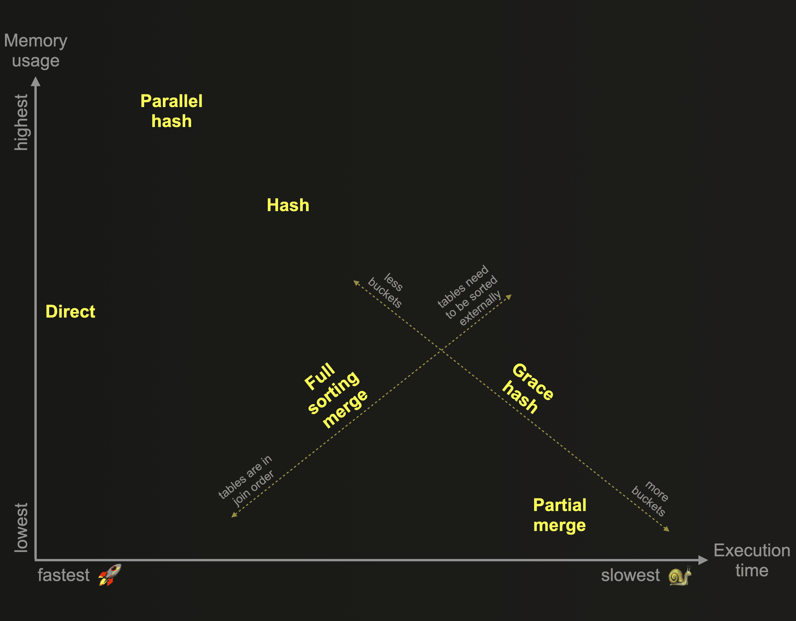
Selecting the right join algorithm is crucial for optimizing join performance in ClickHouse. The choice depends on factors such as table sizes, available memory, and query patterns.

By default, ClickHouse uses the hash join algorithm, which is efficient for small to medium-sized tables. However, for larger tables or when memory is limited, you may need to consider other algorithms like the merge join or the nested loop join.

The following chart provides a visual guide of the tradeoffs of the different join algorithms.

Optimize join keys

The choice of join keys can significantly impact join performance. When possible, use integer or fixed-string types for join keys, as they are more efficient compared to variable-length strings or complex data types.

Ensure that the join keys are in the sorting key in both tables to enable faster lookups during the join operation.

Minimize data transfer in distributed joins

When working with distributed tables in ClickHouse, it's important to minimize data transfer during join operations to reduce network overhead and improve performance.

One way to achieve this is by using local joins whenever possible. Local joins are performed on each shard independently, without the need for data transfer between shards. This can significantly reduce network traffic and improve query performance.

Consider data locality when designing distributed schemas. Try to co-locate related data on the same shards to minimize the need for cross-shard data transfer during joins.

Leverage join_use_nulls setting

The join_use_nulls setting in ClickHouse allows you to use NULL values for non-matching rows instead of default values during join operations. Enabling this setting can improve performance and reduce memory usage in certain scenarios.

By default, when there is no match for a row in the left table during a LEFT JOIN or FULL JOIN, ClickHouse fills the non-matching columns with default values. However, when join_use_nulls is enabled, ClickHouse uses NULL values instead.

Utilize `join_any_take_last_row` setting

The join_any_take_last_row setting in ClickHouse is useful when you want to deduplicate data during join operations. When enabled, this setting ensures that only the last matching row is used in ANY JOIN operations.

By default, ANY JOIN returns the first matching row encountered during the join. However, in some cases, you may want to use the last matching row instead. Enabling the join_any_take_last_row setting allows you to achieve this behavior.

Set `join_algorithm='auto'` for adaptive optimization

ClickHouse provides an adaptive join optimization feature through the join_algorithm='auto' setting. When enabled, this setting allows ClickHouse to automatically choose the best join algorithm based on runtime conditions.

With join_algorithm='auto', ClickHouse starts with the hash join algorithm and monitors the memory consumption during the join operation. If the memory usage exceeds the specified limits (max_bytes_in_join or max_rows_in_join), ClickHouse dynamically switches to the partial merge join algorithm to reduce memory pressure.

Consider denormalization for frequently joined data

Denormalization is a technique where redundant data is intentionally introduced to improve query performance. In the context of joins, denormalization involves creating materialized views or pre-joined tables for frequently accessed join patterns.

By denormalizing data, you can reduce the need for expensive join operations at query time. The trade-off is increased storage requirements and potential data inconsistency, which needs to be managed through appropriate update mechanisms.

Conclusion

Alright, let's wrap this up! Joins in ClickHouse might seem like a beast to tackle at first, but trust me, they're not as complex as they appear. Once you get the hang of them, you'll be joining tables like a pro.

Taking the time to learn these joins is totally worth it. They're your secret weapon for combining data from multiple tables, helping you uncover insights that would otherwise stay hidden.

And here's a pro tip: combine joins with materialized views, and you've got yourself a performance powerhouse. It's like turbocharging your queries!

You can get started with Propel's Serverless ClickHouse today and receive $15 in monthly credits forever. At any point, upgrade to pay-as-you-go, or contact us to learn more about our volume-based discounts. Visit our pricing page for details.

Parsing dates in ClickHouse

This is some text inside of a div block.

Heading 1

Heading 2

Heading 3

Heading 4

Heading 5

Heading 6

Lorem ipsum dolor sit amet, consectetur adipiscing elit, sed do eiusmod tempor incididunt ut labore et dolore magna aliqua. Ut enim ad minim veniam, quis nostrud exercitation ullamco laboris nisi ut aliquip ex ea commodo consequat. Duis aute irure dolor in reprehenderit in voluptate velit esse cillum dolore eu fugiat nulla pariatur.